2020.04.16

【PyTorch】Guided Grad CAMによるCNNの可視化

CNN Deconvnet GradCAM Guided backpropagation Guided GradCAM pytorch VGG16 画像認識

Guided GradCAMをpytorchを用いて実装する

前回、CNNの注目箇所の可視化手法として、GradCAMを実装しました。
今回はGradCamの論文でGradCAMと共に提案されているGuided GradCAMを実装します。
Guided GradCAMはGrad CAMより解像度を高く注目箇所を可視化する方法として提案されています。

# 使用するライブラリの読み込み
import torch
import torch.nn as nn
import torch.nn.functional as F
from torch import optim
import pandas as pd
import numpy as np
import matplotlib.pyplot as plt
from torchvision import datasets, transforms
from torchvision import models
from tqdm import tqdm_notebook as tqdm
from PIL import Image
import cv2
device = torch.device("cuda" if torch.cuda.is_available() else "cpu")

モデル、データ読み込み

前回同様モデルは学習済みモデルVGG16を利用します。
学習済みモデルの読み込み、予測の詳細については前回のブログを確認ください。

feature_extractor = models.vgg16(pretrained=True).features
classifier = models.vgg16(pretrained=True).classifier
# 次の平均、分散を用いて正規化
normalize = transforms.Normalize(
    mean=[0.485, 0.456, 0.406],
    std=[0.229, 0.224, 0.225])
# 画像の正規化を戻すのに利用します
mean = torch.tensor([0.485, 0.456, 0.406]).view(3,1,1)
std = torch.tensor([0.229, 0.224, 0.225]).view(3,1,1)
# 画像を256x256にリサイズ　→　中央の224を切り取り
preprocess = transforms.Compose([
    transforms.Resize(256),
    transforms.CenterCrop(224),
    transforms.ToTensor(),
    normalize
])
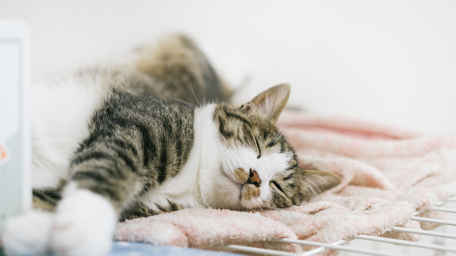
img = Image.open('/content/drive/My Drive/Colab Notebooks/cat_img.jpg')
# 画像の正規化
img_tensor = preprocess(img)

画像も前回同様猫の画像を使用します

img

GradCAMの確認

前回実装した、出力を確認しておきます。

# グレースケールをヒートマップにする関数
# 得られたグレースケールの注目箇所をヒートマップに変換する際に用います
def toHeatmap(x):
    x = (x*255).reshape(-1)
    cm = plt.get_cmap('jet')
    x = np.array([cm(int(np.round(xi)))[:3] for xi in x])
    return x.reshape(224,224,3)
feature = feature_extractor(img_tensor.view(-1,3,224,224)) #特徴マップを計算
feature = feature.clone().detach().requires_grad_(True) #勾配を計算するようにコピー
y_pred = classifier(feature.view(-1,512*7*7)) #予測を行う
y_pred[0][torch.argmax(y_pred)].backward() # 予測でもっとも高い値をとったクラスの勾配を計算
# 以下は上記の式に倣って計算しています
alpha = torch.mean(feature.grad.view(512,7*7),1)
feature = feature.view(512,7,7)
L = F.relu(torch.sum(feature*alpha.view(-1,1,1),0)).cpu().detach().numpy()
# (0,1)になるように正規化
L_min = np.min(L)
L_max = np.max(L - L_min)
L = (L - L_min)/L_max
# 得られた注目度をヒートマップに変換
L = toHeatmap(cv2.resize(L,(224,224)))
img1 = (img_tensor*std + mean).permute(1,2,0).cpu().detach().numpy()
img2 = L
alpha = 0.3
blended = img1*alpha + img2*(1-alpha)
# 結果を表示する。
plt.figure(figsize=(10,10))
plt.imshow(blended)
plt.axis('off')
plt.show()

大まかに、体と耳に注目していることがわかりますが、より詳細に耳や体のどこを見ているかは確認できません。そこで今回の目的のGuided GradCAMが登場します。
ちなみに、VGG16でこの猫を識別すると’tabby cat’('トラ猫')となるので分類は適切に行えています。

Guided GradCAM

Guided GradCAMはguided backpropagationとGradCAMの出力を組み合わせたものになります。
また、guided backpropagationはDeconvnetというCNNの可視化技術を発展させたものでDeconvnetよりぼやけない出力が得られると言われています。

まず、Deconvnetについて説明し、guidedbackpropagation、Guided GradCAMと説明していきます。

Deconvnet

Deconvnetの解説についてはこちらの記事がよくまとまっています。

Deconvnetは次の図で表現されます。

https://arxiv.org/abs/1311.2901　より

畳み込み→ReLU関数→MaxPoolingと畳み込まれたものを
MaxUnPooling→ReLU関数→転置畳み込み
とすることで得られた特徴マップを復元しようと考えれたネットワークになります。

次のようにモデルは設計されます。

簡略化のためConv -> ReLUとReLU -> ConvTranspose は一つのクラスにしておきます。

class CR(nn.Module):
    def __init__(self,in_ch,out_ch):
        super(CR,self).__init__()
        self.cr = nn.Sequential(nn.Conv2d(in_ch,out_ch,3,1,1),nn.ReLU(inplace=True))
    def forward(self,x):
        return self.cr(x)
class RC(nn.Module):
    def __init__(self,in_ch,out_ch):
        super(RC,self).__init__()
        self.rc = nn.Sequential(nn.ReLU(inplace=True),nn.ConvTranspose2d(in_ch,out_ch,3,1,1))
    def forward(self,x):
        return self.rc(x)

特徴マップを生成する部分と逆伝播を行う部分での
パラメータ共有を記述した部分と学習済みパラメータの読み込みで
多少モデルが長くなってしまっています

class Deconvnet(nn.Module):
    def __init__(self):
        super(Deconvnet,self).__init__()
        #　特徴マップを生成する部分
        self.conv1 = nn.Sequential(CR(3,64),CR(64,64),nn.MaxPool2d(2,return_indices=True))
        self.conv2 = nn.Sequential(CR(64,128),CR(128,128),nn.MaxPool2d(2,return_indices=True))
        self.conv3 = nn.Sequential(CR(128,256),CR(256,256),CR(256,256),nn.MaxPool2d(2,return_indices=True))
        self.conv4 = nn.Sequential(CR(256,512),CR(512,512),CR(512,512),nn.MaxPool2d(2,return_indices=True))
        self.conv5 = nn.Sequential(CR(512,512),CR(512,512),CR(512,512),nn.MaxPool2d(2,return_indices=True))
        # 特徴マップを逆伝播する部分
        self.deconv5 = nn.Sequential(RC(512,512),RC(512,512),RC(512,512))
        self.deconv4 = nn.Sequential(RC(512,512),RC(512,512),RC(512,256))
        self.deconv3 = nn.Sequential(RC(256,256),RC(256,256),RC(256,128))
        self.deconv2 = nn.Sequential(RC(128,128),RC(128,64))
        self.deconv1 = nn.Sequential(RC(64,64),RC(64,3))
        self.unpool5 = nn.MaxUnpool2d(2)
        self.unpool4 = nn.MaxUnpool2d(2)
        self.unpool3 = nn.MaxUnpool2d(2)
        self.unpool2 = nn.MaxUnpool2d(2)
        self.unpool1 = nn.MaxUnpool2d(2)
        # 学習済みパラメータの読み込み
        self.conv1[0].cr[0].weight = feature_extractor[0].weight
        self.conv1[1].cr[0].weight = feature_extractor[2].weight
        self.conv2[0].cr[0].weight = feature_extractor[5].weight
        self.conv2[1].cr[0].weight = feature_extractor[7].weight
        self.conv3[0].cr[0].weight = feature_extractor[10].weight
        self.conv3[1].cr[0].weight = feature_extractor[12].weight
        self.conv3[2].cr[0].weight = feature_extractor[14].weight
        self.conv4[0].cr[0].weight = feature_extractor[17].weight
        self.conv4[1].cr[0].weight = feature_extractor[19].weight
        self.conv4[2].cr[0].weight = feature_extractor[21].weight
        self.conv5[0].cr[0].weight = feature_extractor[24].weight
        self.conv5[1].cr[0].weight = feature_extractor[26].weight
        self.conv5[2].cr[0].weight = feature_extractor[28].weight
        # パラメータ共有の記述
        self.deconv1[1].rc[1].weight = feature_extractor[0].weight
        self.deconv1[0].rc[1].weight = feature_extractor[2].weight
        self.deconv2[1].rc[1].weight = feature_extractor[5].weight
        self.deconv2[0].rc[1].weight = feature_extractor[7].weight
        self.deconv3[2].rc[1].weight = feature_extractor[10].weight
        self.deconv3[1].rc[1].weight = feature_extractor[12].weight
        self.deconv3[0].rc[1].weight = feature_extractor[14].weight
        self.deconv4[2].rc[1].weight = feature_extractor[17].weight
        self.deconv4[1].rc[1].weight = feature_extractor[19].weight
        self.deconv4[0].rc[1].weight = feature_extractor[21].weight
        self.deconv5[2].rc[1].weight = feature_extractor[24].weight
        self.deconv5[1].rc[1].weight = feature_extractor[26].weight
        self.deconv5[0].rc[1].weight = feature_extractor[28].weight
    def forward(self,x):
        x,p1 = self.conv1(x)
        x,p2 = self.conv2(x)
        x,p3 = self.conv3(x)
        x,p4 = self.conv4(x)
        x,p5 = self.conv5(x)
        return x
    def deconv(self,x):
        x,p1 = self.conv1(x)
        x,p2 = self.conv2(x)
        x,p3 = self.conv3(x)
        x,p4 = self.conv4(x)
        x,p5 = self.conv5(x)
        x = self.deconv5(self.unpool5(x,p5))
        x = self.deconv4(self.unpool4(x,p4))
        x = self.deconv3(self.unpool3(x,p3))
        x = self.deconv2(self.unpool2(x,p2))
        x = self.deconv1(self.unpool1(x,p1))
        return x

上記のモデルを実装し、出力する

deconvnet = Deconvnet()
deconvnet = deconvnet.eval()
map1 = deconvnet.deconv(img_tensor.view(-1,3,224,224))[0].permute(1,2,0).cpu().detach().numpy()
# 値が[0,1]になるように正規化
map1_min = np.min(map1)
map1_max = np.max(map1 - map1_min)
map1 = (map1 - map1_min)/map1_max
plt.figure(figsize=(10,10))
plt.imshow(map1)

ノイズが入っているが、猫の輪郭や、目、耳が強調されていることが確認できる

guided backpropagation

guided backpropagationは次の図で説明されます。

https://arxiv.org/abs/1412.6806　より

Deconvnetに加え、特徴マップを生成する際のReLU関数で活性化された場所を記憶し、
その場所のみを逆伝播させるモデルになります。

モデルの記述は上記のDeconvnetにReLU関数の活性化した場所を記憶する記述を加えたので、
より長くなってしまっています。

class Guided_backpropagation(nn.Module):
    def __init__(self):
        super(Guided_backpropagation,self).__init__()
        #　特徴マップを生成する部分
        self.conv1 = nn.Sequential(CR(3,64),CR(64,64),nn.MaxPool2d(2,return_indices=True))
        self.conv2 = nn.Sequential(CR(64,128),CR(128,128),nn.MaxPool2d(2,return_indices=True))
        self.conv3 = nn.Sequential(CR(128,256),CR(256,256),CR(256,256),nn.MaxPool2d(2,return_indices=True))
        self.conv4 = nn.Sequential(CR(256,512),CR(512,512),CR(512,512),nn.MaxPool2d(2,return_indices=True))
        self.conv5 = nn.Sequential(CR(512,512),CR(512,512),CR(512,512),nn.MaxPool2d(2,return_indices=True))
        # 　逆伝播を行う部分
        self.deconv5 = nn.Sequential(RC(512,512),RC(512,512),RC(512,512))
        self.deconv4 = nn.Sequential(RC(512,512),RC(512,512),RC(512,256))
        self.deconv3 = nn.Sequential(RC(256,256),RC(256,256),RC(256,128))
        self.deconv2 = nn.Sequential(RC(128,128),RC(128,64))
        self.deconv1 = nn.Sequential(RC(64,64),RC(64,3))
        self.unpool5 = nn.MaxUnpool2d(2)
        self.unpool4 = nn.MaxUnpool2d(2)
        self.unpool3 = nn.MaxUnpool2d(2)
        self.unpool2 = nn.MaxUnpool2d(2)
        self.unpool1 = nn.MaxUnpool2d(2)
        # 学習済みパラメータを読み込む部分
        self.conv1[0].cr[0].weight = feature_extractor[0].weight
        self.conv1[1].cr[0].weight = feature_extractor[2].weight
        self.conv2[0].cr[0].weight = feature_extractor[5].weight
        self.conv2[1].cr[0].weight = feature_extractor[7].weight
        self.conv3[0].cr[0].weight = feature_extractor[10].weight
        self.conv3[1].cr[0].weight = feature_extractor[12].weight
        self.conv3[2].cr[0].weight = feature_extractor[14].weight
        self.conv4[0].cr[0].weight = feature_extractor[17].weight
        self.conv4[1].cr[0].weight = feature_extractor[19].weight
        self.conv4[2].cr[0].weight = feature_extractor[21].weight
        self.conv5[0].cr[0].weight = feature_extractor[24].weight
        self.conv5[1].cr[0].weight = feature_extractor[26].weight
        self.conv5[2].cr[0].weight = feature_extractor[28].weight
        # パラメータ共有を記述する部分
        self.deconv1[1].rc[1].weight = feature_extractor[0].weight
        self.deconv1[0].rc[1].weight = feature_extractor[2].weight
        self.deconv2[1].rc[1].weight = feature_extractor[5].weight
        self.deconv2[0].rc[1].weight = feature_extractor[7].weight
        self.deconv3[2].rc[1].weight = feature_extractor[10].weight
        self.deconv3[1].rc[1].weight = feature_extractor[12].weight
        self.deconv3[0].rc[1].weight = feature_extractor[14].weight
        self.deconv4[2].rc[1].weight = feature_extractor[17].weight
        self.deconv4[1].rc[1].weight = feature_extractor[19].weight
        self.deconv4[0].rc[1].weight = feature_extractor[21].weight
        self.deconv5[2].rc[1].weight = feature_extractor[24].weight
        self.deconv5[1].rc[1].weight = feature_extractor[26].weight
        self.deconv5[0].rc[1].weight = feature_extractor[28].weight
    def forward(self,x):
        x,p1 = self.conv1(x)
        x,p2 = self.conv2(x)
        x,p3 = self.conv3(x)
        x,p4 = self.conv4(x)
        x,p5 = self.conv5(x)
        return x
    def deconv(self,x):
        # xが伝播される特徴マップ
        # rがReLUの活性化の場所
        # pがMaxPoolingの場所
        x = self.conv1[0](x)
        r11 = torch.sign(x)
        x = self.conv1[1](x)
        r12 = torch.sign(x)
        x,p1 = self.conv1[2](x)
        x = self.conv2[0](x)
        r21 = torch.sign(x)
        x = self.conv2[1](x)
        r22 = torch.sign(x)
        x,p2 = self.conv2[2](x)
        x = self.conv3[0](x)
        r31 = torch.sign(x)
        x = self.conv3[1](x)
        r32 = torch.sign(x)
        x = self.conv3[2](x)
        r33 = torch.sign(x)
        x,p3 = self.conv3[3](x)
        x = self.conv4[0](x)
        r41 = torch.sign(x)
        x = self.conv4[1](x)
        r42 = torch.sign(x)
        x = self.conv4[2](x)
        r43 = torch.sign(x)
        x,p4 = self.conv4[3](x)
        x = self.conv5[0](x)
        r51 = torch.sign(x)
        x = self.conv5[1](x)
        r52 = torch.sign(x)
        x = self.conv5[2](x)
        r53 = torch.sign(x)
        x,p5 = self.conv5[3](x)
        x = self.deconv5[2](r51*self.deconv5[1](r52*self.deconv5[0](r53*self.unpool5(x,p5))))
        x = self.deconv4[2](r41*self.deconv4[1](r42*self.deconv4[0](r43*self.unpool4(x,p4))))
        x = self.deconv3[2](r31*self.deconv3[1](r32*self.deconv3[0](r33*self.unpool3(x,p3))))
        x = self.deconv2[1](r21*self.deconv2[0](r22*self.unpool2(x,p2)))
        x = self.deconv1[1](r11*self.deconv1[0](r12*self.unpool1(x,p1)))
        return x

guided_backpropagation = Guided_backpropagation()
guided_backpropagation = guided_backpropagation.eval()
map2 = guided_backpropagation.deconv(img_tensor.view(-1,3,224,224))[0].permute(1,2,0).cpu().detach().numpy()
map2_min = np.min(map2)
map2_max = np.max(map2 - map2_min)
map2 = (map2 - map2_min)/map2_max
plt.figure(figsize=(10,10))
plt.imshow(map2)

Deconvnetと比較してノイズがなくなり、トラ猫の特徴であるシマシマや猫の特徴のひげ、耳等が注目されていることがわかる。

Guided GradCAMの実装

上記で猫の詳細などの部分を見ているかguided backpropagationにより確認できたが、猫全体が強調され、どの部分を見ているかがぼやけてしまっている。
そこで、場所を捉えることができるGradCAMと詳細を捉えるguided backpropagationを組み合わせ注目箇所を可視化する手法がGuided GradCAMである

## ヒートマップに変換しないGradCAMの出力を得る
feature = feature_extractor(img_tensor.view(-1,3,224,224)) #特徴マップを計算
feature = feature.clone().detach().requires_grad_(True) #勾配を計算するようにコピー
y_pred = classifier(feature.view(-1,512*7*7)) #予測を行う
y_pred[0][torch.argmax(y_pred)].backward() # 予測でもっとも高い値をとったクラスの勾配を計算
# 以下は上記の式に倣って計算しています
alpha = torch.mean(feature.grad.view(512,7*7),1)
feature = feature.view(512,7,7)
L = F.relu(torch.sum(feature*alpha.view(-1,1,1),0)).cpu().detach().numpy()
# (0,1)になるように正規化
L_min = np.min(L)
L_max = np.max(L - L_min)
L = (L - L_min)/L_max
L = cv2.resize(L,(224,224))
plt.figure(figsize=(6,6))
plt.imshow(L,cmap='gray')

上記の白くなっている場所が場所として注目しているGradCAMの出力になります、これと
先ほどのguided backpropagationの出力を組み合わせると次のようになります。

map3 = L.reshape(224,224,1)*map2
plt.figure(figsize=(10,10))
plt.imshow(map3)

組み合わせることで、猫のシマシマと、右目から右耳付け根を注目していることが確認できる。

前回の記事の最後に、attentionを可視化したいと書きましたがbackpropagationになってしまいました。また時間があればattentionの可視化についても書いていきたいと思います。

\ いいなと思ったらシェア /

ブログトップに戻る

【PyTorch】Guided Grad CAMによるCNNの可視化

Guided GradCAMをpytorchを用いて実装する

モデル、データ読み込み

GradCAMの確認

Guided GradCAM

Deconvnet

guided backpropagation

Guided GradCAMの実装

DCGANで実家のﾈｺﾁｬﾝの画像を生成しようとしたら成れ果てになった【後編】

PyTorch Geometric(GNN)のインストール方法

学習中に「cunDNN error : CUDNN_STATUS_MAPPING_ERROR」が出た

最近の投稿

【PyTorch】Guided Grad CAMによるCNNの可視化

Guided GradCAMをpytorchを用いて実装する

モデル、データ読み込み

GradCAMの確認

Guided GradCAM

Deconvnet

guided backpropagation

Guided GradCAMの実装

関連記事

DCGANで実家のﾈｺﾁｬﾝの画像を生成しようとしたら成れ果てになった【後編】

PyTorch Geometric(GNN)のインストール方法

学習中に「cunDNN error : CUDNN_STATUS_MAPPING_ERROR」 が出た

検索

人気記事

最近の投稿

タグ

学習中に「cunDNN error : CUDNN_STATUS_MAPPING_ERROR」が出た